This page explains how to use a hinged tiling proceedure to obtain (in the limit)
a space filling curve.
The program here
can be used to generate lots of pictures using this idea.
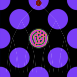
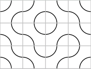
First, start with a tiling consisting of tiles with quarter circles at opposite corners,
like this (though other tiles can be used). Left is a png image;
click on right image
for change of orientation of tiles.
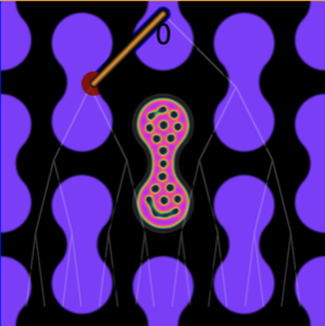
Next hinge the tiling, in one of two ways,
and when maximally opened, fill in in the unique
way to preseve the connected componenets, i.e., things join up in the same way,
like this (left is fixed; use this slider to alter right
)
:
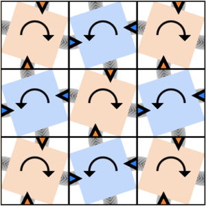
The following picture is to make clear the regular pattern that the added tiles
appear in, in both cases. The blue squares turn anticlockwise, and orange squares turn
clockwise.
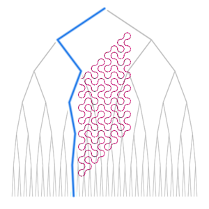
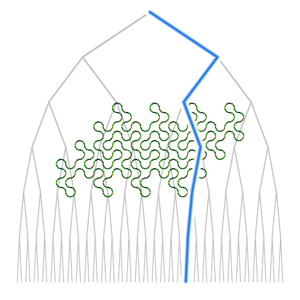
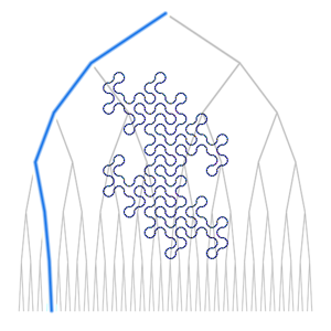
See also this picture. There are two possible choices of this operation, and the operation can be applied over and over again, according to a binary choice, so we get a choice tree, and possible outcomes as in the following examples.
These curves can be considered as L-systems.
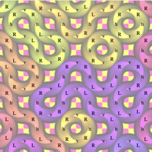
For each curve, we can give an instruction for the path, e.g., as in the following picture:
L means turn left, R means turn right, h means cross a horizontal line, v means cross a
vertical line.
The hinged tiling process corresponds to either:
L → L ,
R → R ,
h → hLv,
v → hRv
or
L → L ,
R → R ,
h → hRv ,
v → hLv
You can see this by looking at the following picture, and see how in this picture,
the little orange arrows which appear in the horizontal gaps all point to the right, and
the blue arrows in the vertical gaps point to the left. The directions followed on the
rotated squares do not change.
The second of these operations is illustrated in the following program. You can
move the slider from 0 to 1 to go from the initial configuration to the
new configuration.
Apply operation:
0
As the iterations increase, the curve will get arbitrarily close to any point, so is
space filling in the limit. At the extremes are the fractal dragon curve, and the
curve with overall parallelogram shape above.
Here are a few pictures illustrating the relationship between one level of iteration and the next, by including succesive steps superimposed.
The first shows curves, as in the original tile; the others show the curve replaced by a
straight line, with end point the same as on the initial tile.
These were made with this program.
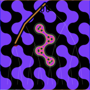
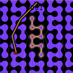
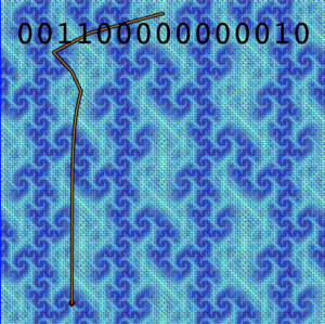
The following show the first few steps of a sequence of choices, from the empty choice,
through 0,00,001,0011
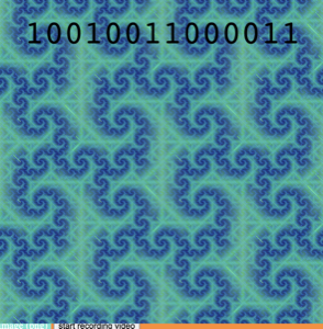
These are pictures of the fractals obtained after up to 15 itterations, with the
curves up to the given level superimposed.
Here are all the cases after 4 steps
Here are all the cases after 15 steps (or here (mp4),
(webm),
in case
below doesn&apos t work):
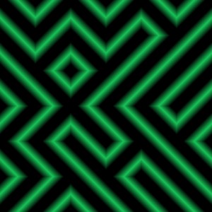
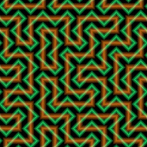
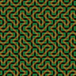
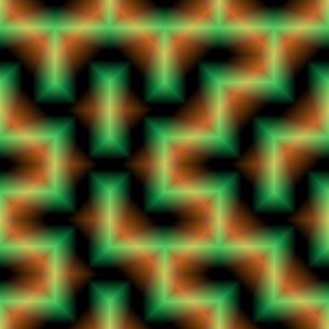
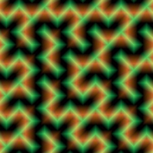
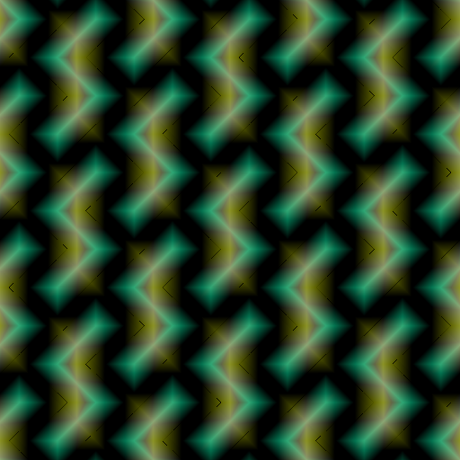
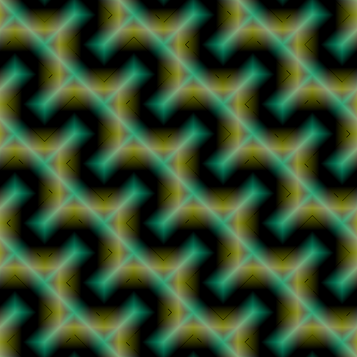
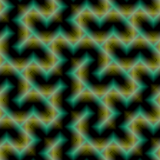
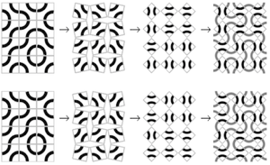
Here is another sequence of pictures showing the progression of the iterative
process. In this case, the basic tile has two diagonal lines instead of the two quarter circles, so the first picture on the left below shows at 6x6 array of these tiles
in random configuration. In this sequence of pictures, at each stage the green lines of one figure are replaced by red lines in the next, and the next step is drawn over in green.
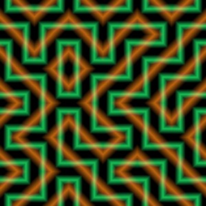
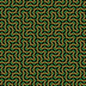
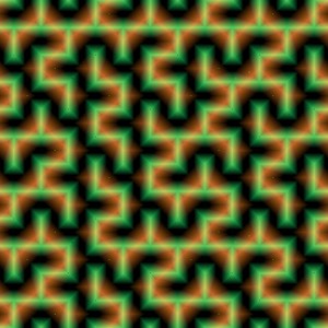
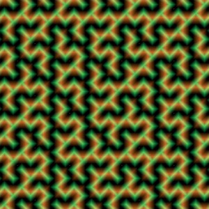
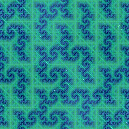
For comparision, here is the filled in version of the above sequence:
Note, for a filled in version, there is a rule for how tiles transform:
even tiles with zero rotation and odd tiles with 90 degrees rotation have the
section between the two lines coloured, and for the other tiles it&apos s the reverse
situation.
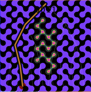
SVG L-system version
The above images are all produced by Webgl. Here is an svg version.
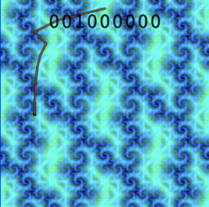
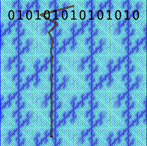
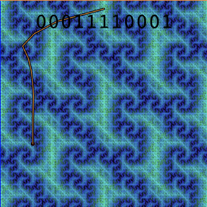
Type in a sequence of 0s and 1s to indicate which sequence of operations is applied.
A maximum of 15 characters is allowed.
This version of drawing these curves just uses the L-system method, in a very simple
way, starting from a little dot.
There is some automatic translation to try and centre the curve.
The initial
configuration corresponds to 0000000000 applied RhRvRhRv.
Use L and R to change the initial string in the box provided.
The program inserts the h and v which are used in
determining the L-system process. Note that when you enter
l and r etc, the program does not check this corresponds to a
possible path created by a Trouchet tiling, so this may result in
overlapping situations. If you only enter a sequence obtainable from
a Trouchet arrangement, and the path does not repeat over itself,
you get a nonoverlapping path, because you only
ever get a Trouchet tiling arangement, and these have no overlaps.
Note that at most four colours are enough to colour so that adjacent tiles
(derived from distinct initial line segements) do not touch if they are the same colour (except possibly in a limiting sense at corners) if following trouchet
path. Also note that only strings of length at most 100 will work in this
implementation. If strings are too long, results may be incorrect, since
the program will stop computing, but does not warn you.
The starting point of the path is marked with a red dot.
Unfortunately it appears I got L and R mixed up.
Fixed in code, I think.
Also there are some bugs in some cases for the latex.
for the output, because of latex orientation of
y-axis being opposite of svg direction, and I have not completely taken
account of this yet, the latex may sometimes be upsidedown. Note that
the latex produces a standalone latex tikzpicture file you can compile with
your favourite latex compiler.
Note that scale for latex is not using the same function as scale for svg,
which may lead to unexpected results.
also problem currently with scale keeps getting reset
The above system corresponds to taking the following Trouchet tile
(change using "tile option" selection above):
The initial configuration corresponds to taking four of these tiles together, shown slightly apart here, so we can distinguish tiles. Then for the iteration
above, we only use the middle componenets, and forget about the other half of each tile.
We can vary the exact path, using the choice selection above to see examples,
but the end points, marked
by the black dots, are the same in all these cases, and in the limit the
curve we get is going to be the same, and the exact path chosen
between the end points won&apos t really matter.
Use the "all combined" option to see all tiles at once for comparision.
Comparision with usual fractal dragon
The fractal dragon curve here is slightly different from the standard
definition, e.g., at
Wikipedia page on fractal dragon.
The difference is because here we use a union of four segments, so actually
we get a union of four fractal dragon curves.
I have coloured these in four different colours to distinguish them.
The basic dragon curve comes from taking just one of these, and the twin dragon would be from 2 copies of this.
The usual fractal dragon corresponds to taking the third choice of tile, and
the binary sequence "00000...".
Also, in the L-system, here
we interpret "L" or "R" as "go left/right while moving", rather than turning
and moving as two separate things. This means that the difference in the
path compared with usual curve just means subtract half
the first segment of the
path here, and add to the end of the path the first
half segment of the next path.
To see the usual fractal dragon construction, use the fourth option for
type of tile, "straight line", which really is a line crossing tiles, if we
want to view the construction in the context of hinged tilings.
Arbitrary initial tile orientation
Most of the above pictures use the same simple initial tiling of circles, but these
methods apply to any initial Trouchet tiling of the quarter circle or diagonal line
tile.
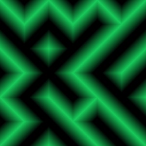
These three pictures show example of the process applied, just one step,
to three different initial tiles.
This picture has several applications of the process to an initial random tiling
of Trouchet tiles with two parallel diagonal lines.

.png)
.png)
.png)
.png)